Diffusion models II: DDPMs, NCSNs and score-based generative modelling using SDEs

The following case study introduces recent developments in generative modelling using diffusion models. We will first introduce two landmark papers on diffusion models, “Denoising Diffusion Probabilistic Models” (Ho, Jain, and Abbeel 2020) and “Generative Modeling by Estimating Gradients of the Data Distribution” (Song and Ermon 2019), and then examine a general framework introduced in Song et al. (2021) that unifies both. This case study is the second in a series on diffusion models: please find the first one here.

We’ll reimplement all three vanilla models using Jax, Haiku and Optax.

Code

import warnings
warnings.filterwarnings("ignore")

from dataclasses import dataclass

import distrax
import haiku as hk
import numpy as np
import jax
import optax
import pandas as pd
from jax import lax, nn, jit, grad
from jax import numpy as jnp
from jax import random
from jax import scipy as jsp
from scipy import integrate

import arviz as az
import matplotlib.pyplot as plt
import palettes
import seaborn as sns

sns.set(rc={"figure.figsize": (6, 3)})
sns.set_style("ticks", {"font.family": "serif", "font.serif": "Merriweather"})
palettes.set_theme()

DDPMs

As discussed in the first part of the series, diffusion models (Sohl-Dickstein et al. 2015) are a class of generative models of the form

\[ p_\theta \left( \mathbf{y}_0 \right) = \int p_\theta \left( \mathbf{y}_0, \mathbf{y}_{1:T} \right) d\mathbf{y}_{1:T} \]

where every transition \(p_\theta(\mathbf{y}_{t-1} \mid \mathbf{y}_{t})\) is parameterized by the same neural network \(\theta\) and trained by optimizing a lower bound on the marginal log-likelihood:

\[\begin{align*} \log p_\theta(\mathbf{y}_0) \ge \mathbb{E}_{q(\mathbf{y}_{1:T})} \Bigl[ & \log p_\theta(\mathbf{y}_0 \mid \mathbf{y}_{1}) \\ &+ \sum_{i=1}^{T - 1} \log p_\theta(\mathbf{y}_i \mid \mathbf{y}_{i + 1}) - \sum_{i=2}^{T} \log q(\mathbf{y}_i \mid \mathbf{y}_{i - 1}) \\ & + \log p_\theta(\mathbf{y}_T) - \log q(\mathbf{y}_1 \mid \mathbf{y}_0) \Bigr] \end{align*}\]

In comparison to other latent variables models, DPMs use an approximate posterior \(q\left(\mathbf{y}_{1:T} \mid \mathbf{y}_0 \right) = q(\mathbf{y}_{1} \mid \mathbf{y}_0) \prod_{t=2}^T q(\mathbf{y}_{t} \mid \mathbf{y}_{t - 1})\) that is fixed to a Markov chain and which repeatedly adds noise to the initial data set, while the joint distribution \(p_\theta \left( \mathbf{y}_0, \mathbf{y}_{1:T} \right)\) is learned. As discussed in the previous case study, the ELBO above can be reformulated as

\[\begin{align*} \mathbb{E}_{q} \biggl[ \log p_\theta \left(\mathbf{y}_0 \mid \mathbf{y}_1 \right) - \sum_{t=2}^T \mathbb{KL}\Bigl[ q(\mathbf{y}_{t - 1} \mid \mathbf{y}_{t}, \mathbf{y}_0), p_\theta(\mathbf{y}_{t - 1} \mid \mathbf{y}_t) \Bigr] - \mathbb{KL}\Bigl[ q(\mathbf{y}_T \mid \mathbf{y}_0), p_\theta(\mathbf{y}_T) \Bigr] \biggr] \end{align*}\]

where

\[\begin{align*} q \left( \mathbf{y}_{t - 1} \mid \mathbf{y}_{t}, \mathbf{y}_0 \right) & = \frac{q \left( \mathbf{y}_{t} \mid \mathbf{y}_{t-1} , \mathbf{y}_0 \right) q\left( \mathbf{y}_{t-1} \mid \mathbf{y}_0 \right) }{q \left( \mathbf{y}_{t} \mid \mathbf{y}_0 \right) } \\ & = \mathcal{N} \left( \tilde{\boldsymbol \mu}_t\left( \mathbf{y}_{t}, \mathbf{y}_0\right) , \tilde{\beta}_t \mathbf{I} \right) \end{align*}\]

which can be computed in closed form. The insight from Ho, Jain, and Abbeel (2020) is that the objective above can be simplified (and numerically stabilized) by setting the covariance matrix of the reverse process \(p_\theta \left(\mathbf{y}_{t-1} \mid \mathbf{y}_{t} \right) = \mathcal{N}\left(\boldsymbol \mu_\theta \left(\mathbf{y}_{t}, t\right), \boldsymbol \Sigma(\mathbf{y}_{t}, t)\right)\) to a constant \(\boldsymbol \Sigma \left(\mathbf{y}_{t}, t \right) = \sigma_t^2\mathbf{I}\). The divergence between the forward process posterior and the reverse process can then be written as

\[\begin{align*} L_{t-1} & = \mathbb{E}_{q} \biggl[ \frac{1}{2\sigma_t^2} \| \tilde{\boldsymbol \mu}_t\left(\mathbf{y}_t, \mathbf{y}_0\right) - \boldsymbol \mu_{\theta}\left(\mathbf{y}_t, \mathbf{y_0}\right) \|^2_2 \biggr] + C \end{align*}\]

So, we can parameterize \(\boldsymbol \mu_\theta\) using a model that predicts the forward process posterior mean \(\tilde{\boldsymbol \mu}\). We can further develop this formulation by applying the usual Gaussian reparameterization trick and arrive at an objective that is significantly more stable to optimize than the initial ELBO, but for the sake of this case study we will not derive the math here and refer the read to the original publication.

In practice, we just sample a time point \(t\) and then don’t optimze the entire objective but only

\[\begin{align*} \mathbb{E}_{t, q} \biggl[ \frac{1}{2\sigma_t^2} \| \tilde{\boldsymbol \mu}_t\left(\mathbf{y}_t, \mathbf{y}_0\right) - \boldsymbol \mu_{\theta}\left(\mathbf{y}_t, \mathbf{y}_0\right) \|^2_2 \biggr] \end{align*}\]

where we denote - with a slight abuse of notation - \(t\) as both a time point and the distribution of time points over which the expectation is taken.

To generate new data, we sample first from the prior \(p_T\) and then iteratively denoise the sample until we reach \(p_\theta(\mathbf{y}_0 \mid \mathbf{y}_1)\).

NCSNs

Similarly to DDPMs, noise-conditional score networks (NCSNs, Song and Ermon (2019)) are generative models that make use of noising the data and then trying to train a network that can denoise this process. Unlike DDPMs, NCSNs are motivated through score-matching (Hyvärinen and Dayan 2005) where we are interested in finding a parameterized function \(\mathbf{s}_\theta\) that approximates the score of a data distribution \(q(\mathbf{y})\). Score matching optimizes the following objective

\[\begin{align*} \mathbb{E}_{q(\mathbf{y})} \biggl[ \| \mathbf{s}_\theta(\mathbf{y}) - \nabla_{\mathbf{y}} \log q(\mathbf{y}) ||^2_2 \biggr] \end{align*}\]

In denoising score matching (Vincent 2011), we denoise a data sample with a fixed noise distribution \(q_\sigma \left(\tilde{\mathbf{y}} \mid \mathbf{y} \right) = \mathcal{N}\left(\mathbf{y}, \sigma^2 \mathbf{I} \right)\) to estimate the score of \(q_\sigma \left(\tilde{\mathbf{y}} \right) = \int q_\sigma \left(\tilde{\mathbf{y}} \mid \mathbf{y} \right) p(\mathbf{y})\). Vincent (2011) show that the objective proved equivalent to:

\[\begin{align*} \frac{1}{2}\mathbb{E}_{ q(\mathbf{y}), q_\sigma \left(\tilde{\mathbf{y}} \mid \mathbf{y} \right)} \biggl[ \| \mathbf{s}_\theta\left(\tilde{\mathbf{y}}\right) - \nabla_{\tilde{\mathbf{y}}} \log q_\sigma \left(\tilde{\mathbf{y}} \mid \mathbf{y} \right) ||^2_2 \biggr] \end{align*}\]

In practice, generative modelling using this objective faces two difficulties. One is that if \(\mathbf{y}\) is embedded in a low-dimensional manifold, the gradient taken in the ambient space is undefined. The score estimator is not consistent if the data are residing in a low-dimensional space. Secondly, for regions where there is low data density the score estimator is not accurate.

Song and Ermon (2019) work around both issues by perturbing the data set with multiple levels of noise \(\{ \sigma_i \}_{i=1}^L\) and training a score network that is conditional on the noise levels \(\mathbf{s}\left(\tilde{\mathbf{y}}, \sigma_i \right)\). The authors propose the following objective to train a model of the data:

\[\begin{align*} \frac{1}{2}\mathbb{E}_{\sigma_i, q(\mathbf{y}), q_\sigma \left(\tilde{\mathbf{y}} \mid \mathbf{y} \right)} \biggl[\lambda(\sigma_i) \| \mathbf{s}_\theta\left(\tilde{\mathbf{y}}, \sigma_i\right) - \nabla_{\tilde{\mathbf{y}}} \log q_\sigma \left(\tilde{\mathbf{y}} \mid \mathbf{y} \right) ||^2_2 \biggr] \end{align*}\]

where \(\lambda(\sigma_i)\) is a weighting function that is chosen to be proportional to \(\lambda(\sigma_i) \propto 1 / \mathbb{E}\left[ \|\nabla_{\mathbf{y}} q_\sigma \left(\tilde{\mathbf{y}} \mid \mathbf{y} \|^2_2 \right) \right]\).

To draw samples from the trained model, Song and Ermon (2019) propose using annealed Langevin dynamics where we only need access to the score function of a density to propose new samples (which we just learned).

Score-based SDEs

Before we introduce score-based SDEs, let’s have a look at the DDPM and NCSN objectives again.

Similarities

Let’s first recall that in the DDPM framework we parameterize a model using a neural network \(\boldsymbol \mu_\theta \left(\mathbf{y}_t, t \right)\) to predict the forward process posterior mean \(\tilde{\boldsymbol \mu}\left(\mathbf{y}_t, \mathbf{y}_0 \right) =\frac{\sqrt{\alpha_t}(1 - \bar{\alpha}_{t-1})}{1 - \bar{\alpha}_t} \mathbf{y}_t + \frac{\sqrt{\bar{\alpha}_{t-1} } \beta_t}{1 - \bar{\alpha}_{t}} \mathbf{y}_0\). We recognize that since we actually have access to \(\mathbf{y}_t\), we can alternatively make \(\boldsymbol \mu_\theta \left(\mathbf{y}_t, t \right)\) predict \(\mathbf{y}_0\).

Now, if we recall that \(q(\mathbf{y}_t \mid \mathbf{y}_0) = \mathcal{N}\left(\sqrt{\bar{\alpha_t}} \mathbf{y}_0, \left(1 - \bar{\alpha}_t \right) \mathbf{I} \right)\) and compute the partial derivate of its logarithm w.r.t \(\mathbf{y}_t\)

\[\begin{align*} \nabla_{\mathbf{y}_t} \log q(\mathbf{y}_t \mid \mathbf{y}_0) = - \frac{\mathbf{y}_t - \sqrt{\bar{\alpha_t}} \mathbf{y}_0}{1 - \bar{\alpha}_t} \end{align*}\]

we can see that we can, at least with some algebraic gymnastics, equivalently write

\[\begin{align*} \tilde{\boldsymbol \mu}\left(\mathbf{y}_t, t \right) &= \frac{1}{\sqrt{\alpha_t}} \mathbf{y}_t + \frac{\beta_t}{\sqrt{\alpha_t}} \nabla_{\mathbf{y}_t} \log q(\mathbf{y}_t \mid \mathbf{y}_0) \\ & = \frac{1}{\sqrt{\alpha_t}} \mathbf{y}_t - \frac{\beta_t}{\sqrt{\alpha_t}} \left( \frac{\mathbf{y}_t - \sqrt{\bar{\alpha}_t}\mathbf{y}_0 }{1 - \bar{\alpha}_t} \right) \\ & = \frac{1}{\sqrt{\alpha_t}} \mathbf{y}_t - \frac{\beta_t \mathbf{y}_t}{\sqrt{\alpha_t}\left( 1 - \bar{\alpha}_t\right)} + \frac{\beta_t \sqrt{\bar{\alpha}_t} \mathbf{y}_0}{\sqrt{\alpha_t} \left( 1 - \bar{\alpha}_t\right) } \\ & = \frac{\left( 1 - \bar{\alpha}_t\right)\mathbf{y}_t - \beta_t \mathbf{y}_t}{\sqrt{\alpha_t}\left( 1 - \bar{\alpha}_t\right)} + \frac{\beta_t \sqrt{\bar{\alpha}_{t-1}}}{1 - \bar{\alpha}_t}\mathbf{y}_0 \\ & = \frac{\left( 1 - \bar{\alpha}_t - \beta_t\right)\mathbf{y}_t}{\sqrt{\alpha_t}\left( 1 - \bar{\alpha}_t\right)} + \frac{\beta_t \sqrt{\bar{\alpha}_{t-1}}}{1 - \bar{\alpha}_t}\mathbf{y}_0 \\ & = \frac{\left( 1 - \bar{\alpha}_t - \left(1-\alpha_t\right)\right)\mathbf{y}_t}{\sqrt{\alpha_t}\left( 1 - \bar{\alpha}_t\right)} + \frac{\beta_t \sqrt{\bar{\alpha}_{t-1}}}{1 - \bar{\alpha}_t}\mathbf{y}_0 \\ & = \frac{\alpha_t \left( 1 - \bar{\alpha}_{t-1}\right)\mathbf{y}_t}{\sqrt{\alpha_t}\left( 1 - \bar{\alpha}_t\right)} + \frac{\beta_t \sqrt{\bar{\alpha}_{t-1}}}{1 - \bar{\alpha}_t}\mathbf{y}_0 \\ & = \frac{\sqrt{\alpha_t} \left( 1 - \bar{\alpha}_{t-1}\right)}{1 - \bar{\alpha}_t} \mathbf{y}_t + \frac{\sqrt{\bar{\alpha}_{t-1}}\beta_t }{1 - \bar{\alpha}_t}\mathbf{y}_0 \end{align*}\]

So we can alternatively use a model \(\mathbf{s}_\theta (\mathbf{y}_t, t)\) to predict the score \(\nabla_{\mathbf{y}_t} \log q(\mathbf{y}_t)\) and define the objective:

\[\begin{align*} \mathbb{E}_{t, q(\mathbf{y}_0), q\left(\mathbf{y}_t \mid \mathbf{y}_0 \right)} \biggl[\frac{\lambda(t)}{2} \| \mathbf{s}_\theta\left(\mathbf{y}_t, t\right) - \nabla_{\mathbf{y}_t} \log q \left(\mathbf{y}_t \mid \mathbf{y}_0 \right) ||^2_2 \biggr] \end{align*}\]

where \(\lambda\) is again a weighting function. This makes the relationship between DDPMs and NCSNs obvious, since the denoising score-matching objective is also used in NCSNs.

A common framework

Song et al. (2021) explain that the diffusion processes of DDPMs and NCSNs can be described as an Ito SDE

\[\begin{align*} \mathrm{d} \mathbf{y} = \mathbf{f}(\mathbf{y}, t) \ \mathrm{d}t + g(t) \ \mathrm{d}\mathbf{w} \end{align*}\]

where \(\mathbf{f}\) is called drift coefficient, \(\mathbf{g}\) is called diffusion coefficient and \(\mathbf{w}\) is a Wiener process. The process starts at a data sample \(\mathbf{y}(0) \sim q(\mathbf{y}(0))\) and continuously corrupts it. The DDPM and NCSC are two special discrete-time cases of this process. In case of the DDPM objective, the corresponding SDE is

\[\begin{align*} \mathrm{d} \mathbf{y} = -\frac{1}{2} \beta(t) \mathbf{y} \ \mathrm{d}t + \sqrt{\beta(t)} \ \mathrm{d} \mathbf{w} \end{align*}\]

while for the NCSN we have

\[\begin{align*} \mathrm{d} \mathbf{y} = \sqrt{\frac{\mathrm{d}\sigma^2(t)}{\mathrm{d}t}} \ \mathrm{d}\mathbf{w} \end{align*}\]

These two SDEs specify the forward diffusion processes. We train a score-based SDE by optimising the score matching loss

\[\begin{align*} \frac{1}{2}\mathbb{E}_{t, q(\mathbf{y}(0)), q(\mathbf{y}(t) \mid \mathbf{y}(0))} \biggl[\lambda(t) \| \mathbf{s}_\theta\left(\mathbf{y}(t), t \right) - \nabla_{\mathbf{y}(t)} \log q_{0t} \left(\mathbf{y}(t) \mid \mathbf{y}(0)\right) ||^2_2 \biggr] \end{align*}\]

where \(q_{st}(\mathbf{y}(t) \mid \mathbf{y}(s))\) is a transition kernel that generates \(\mathbf{y}(t)\) from \(\mathbf{y}_s\).

After having trained this objective, we are interested in using the reverse process again to geerate samples. Remarkably, Anderson (1982) state that the reverse of diffusion process is also a diffusion process that runs backward in time. Specifically:

\[\begin{align*} \mathrm{d} \mathbf{y} = \left[ \mathbf{f}(\mathbf{y}, t) - g(t)^2 \nabla_\mathbf{y} \log q_t(\mathbf{y}) \right] \mathrm{d}t + g(t) \mathrm{d}\bar{\mathbf{w} } \end{align*}\]

where \(\bar{\mathbf{w}}\) is a Wiener process that runs reverse in time and \(t\) is a negative timestep. So, in order to train a score-based SDE need to define the forward process. Two options of which are the DDPM and the NCSN, but in general we are free to define any SDE that is a Ito process.

A particularly useful insight fom the paper is that for every diffusion process there exists a corresponding deterministic diffusion process that has the same marginal densitities \(q_t\) as the SDE. This deterministic is an ODE

\[\begin{align*} \mathrm{d} \mathbf{y} = \left[ \mathbf{f}(\mathbf{y}, t) - \frac{1}{2} g(t)^2 \nabla_\mathbf{y} \log q_t(\mathbf{y}) \right] \mathrm{d}t \end{align*}\]

which can be solved using any publically available ODE solver.

Use cases

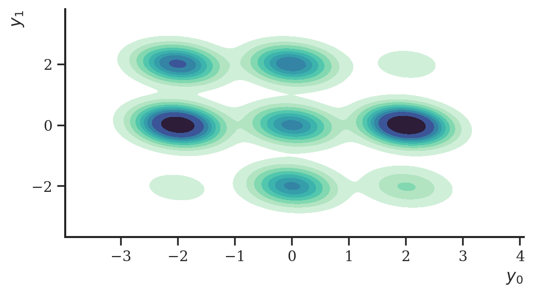
Let’s implement these three models and compare them. We use the nice Gaussians data set again as in the last case study on diffusion models. The nine Gaussians data set is shown below.

Code

K = 9

means = jnp.array([-2.0, 0.0, 2.0])
means = jnp.array(jnp.meshgrid(means, means)).T.reshape(-1, 2)
covs = jnp.tile((1 / 16 * jnp.eye(2)), [K, 1, 1])

probs = distrax.Uniform().sample(seed=random.PRNGKey(23), sample_shape=(K,))
probs = probs / jnp.sum(probs)

d = distrax.MixtureSameFamily(
    distrax.Categorical(probs=probs),
    distrax.MultivariateNormalFullCovariance(means, covs),
)

n = 10000
y = d.sample(seed=random.PRNGKey(12345), sample_shape=(n,))

df = pd.DataFrame(np.asarray(y), columns=["x", "y"])
ax = sns.kdeplot(data=df, x="x", y="y", fill=True, cmap="mako_r")
ax.set_xlabel("$y_0$")
ax.set_ylabel("$y_1$")
plt.show()

Before we start with implementing a model, let’s define an optimizer. We will be able to use the same optimizer for each model.

Code

prng_seq = hk.PRNGSequence(1)
batch_size = 64
num_batches = y.shape[0] // batch_size
idxs = jnp.arange(y.shape[0])

def optim(params, opt_state, n_iter=2000):
    @jax.jit
    def step(params, state, rng, **batch):
        def loss_fn(params):
            loss = model.apply(params, rng, method="loss", is_training=True, **batch)
            return jnp.mean(loss)

        loss, grads = jax.value_and_grad(loss_fn)(params)
        updates, new_state = optimizer.update(grads, state, params)
        new_params = optax.apply_updates(params, updates)
        return loss, new_params, new_state

    losses = [0] * n_iter
    for i in range(n_iter):
        loss = 0.0
        for j in range(batch_size):
            ret_idx = lax.dynamic_slice_in_dim(idxs, j * batch_size, batch_size)
            batch = lax.index_take(y, (ret_idx,), axes=(0,))
            batch_loss, params, opt_state = step(
                params, opt_state, next(prng_seq), y=batch
            )
            loss += batch_loss
        losses[i] = loss
    return params, losses

Score model

We start by implementing a model, i.e., the neural network that estimates the score, noise, etc. We can use the same model for NCSNs, DDPMs, and score-based SDEs. We can also use the same embedding function for the time points and noise levels used in the NCSNs and DDPMs. As a model, we use a simple MLP with gelu activations and a normalisation layer at the end.

from dataclasses import dataclass

def get_embedding(inputs, embedding_dim, max_positions=10000):
    assert len(inputs.shape) == 1
    half_dim = embedding_dim // 2
    emb = jnp.log(max_positions) / (half_dim - 1)
    emb = jnp.exp(jnp.arange(half_dim, dtype=jnp.float32) * -emb)
    emb = inputs[:, None] * emb[None, :]
    emb = jnp.concatenate([jnp.sin(emb), jnp.cos(emb)], axis=1)
    return emb

@dataclass
class ScoreModel(hk.Module):
    output_dim = 2
    hidden_dims = [256, 256]
    embedding_dim = 256

    def __call__(self, z, t, is_training):
        dropout_rate = 0.1 if is_training else 0.0
        t_embedding = jax.nn.gelu(
            hk.Linear(self.embedding_dim)(get_embedding(t, self.embedding_dim))
        )
        h = hk.Linear(self.embedding_dim)(z)
        h += t_embedding

        for dim in self.hidden_dims:
            h = hk.Linear(dim)(h)
            h = jax.nn.gelu(h)

        h = hk.LayerNorm(axis=-1, create_scale=True, create_offset=True)(h)
        h = hk.dropout(hk.next_rng_key(), dropout_rate, h)
        h = hk.Linear(self.output_dim)(h)
        return h

NCSN

We start with the NCSN. The implementation is fairly straight-forward and exactly as described above. It consists of a loss function, and a function to sample new data using annealed Langevin dynamics. We provide a score model and a noise schedule to the constructor and that’s all that is needed.

class NCSN(hk.Module):
    def __init__(self, score_model, sigmata):
        super().__init__()
        self.score_model = score_model
        self.sigmata = sigmata

    def __call__(self, method="loss", **kwargs):
        return getattr(self, method)(**kwargs)

    def loss(self, y, is_training=True):
        def _log_pdf(y, mu, scale):
            scale = jnp.full(mu.shape, scale)
            return distrax.MultivariateNormalDiag(mu, scale).log_prob(y)
        
        stds = random.choice(
            hk.next_rng_key(), 
            a=self.sigmata, 
            shape=(y.shape[0],)
        ).reshape(
            -1,
        )
        noise = random.normal(hk.next_rng_key(), y.shape)
        perturbed_y = y + noise * stds[:, None]
        score = self.score_model(perturbed_y, stds, is_training)
        target = jax.vmap(grad(_log_pdf))(perturbed_y, y, stds[:, None])  
        loss = stds**2 * jnp.sum(jnp.square(score - target), axis=-1)
        return loss

    def sample(self, sample_shape=(1,), n=100, eps=2e-5):
        def _fn(i, z):
            alpha = eps * self.sigmata[i] / self.sigmata[-1]
            sigma = jnp.repeat(self.sigmata[i], z.shape[0])
            for i in jnp.arange(n):
                noise = random.normal(hk.next_rng_key(), z.shape)
                z = (
                    z
                    + 0.5 * alpha * self.score_model(z, sigma, is_training=False)
                    + jnp.sqrt(alpha) * noise
                )
            return z

        z_T = random.normal(hk.next_rng_key(), sample_shape + (2,))
        z0 = hk.fori_loop(0, len(self.sigmata), _fn, z_T)
        return z0

Using Haiku, we need to transform the intialisation of a NCSN object. As a noise schedule, we use a geometric sequence from 1 to 0.01, similarly as to the paper.

def _ncsn(**kwargs):
    score_model = ScoreModel()
    model = NCSN(score_model, jnp.geomspace(1.0, 0.01, 100))
    return model(**kwargs)

model = hk.transform(_ncsn)
params = model.init(random.PRNGKey(0), y=y)

Let’s optimize this and produce some samples.

optimizer = optax.adamw(0.001)
opt_state = optimizer.init(params)

params, losses = optim(params, opt_state)
losses = jnp.asarray(losses)

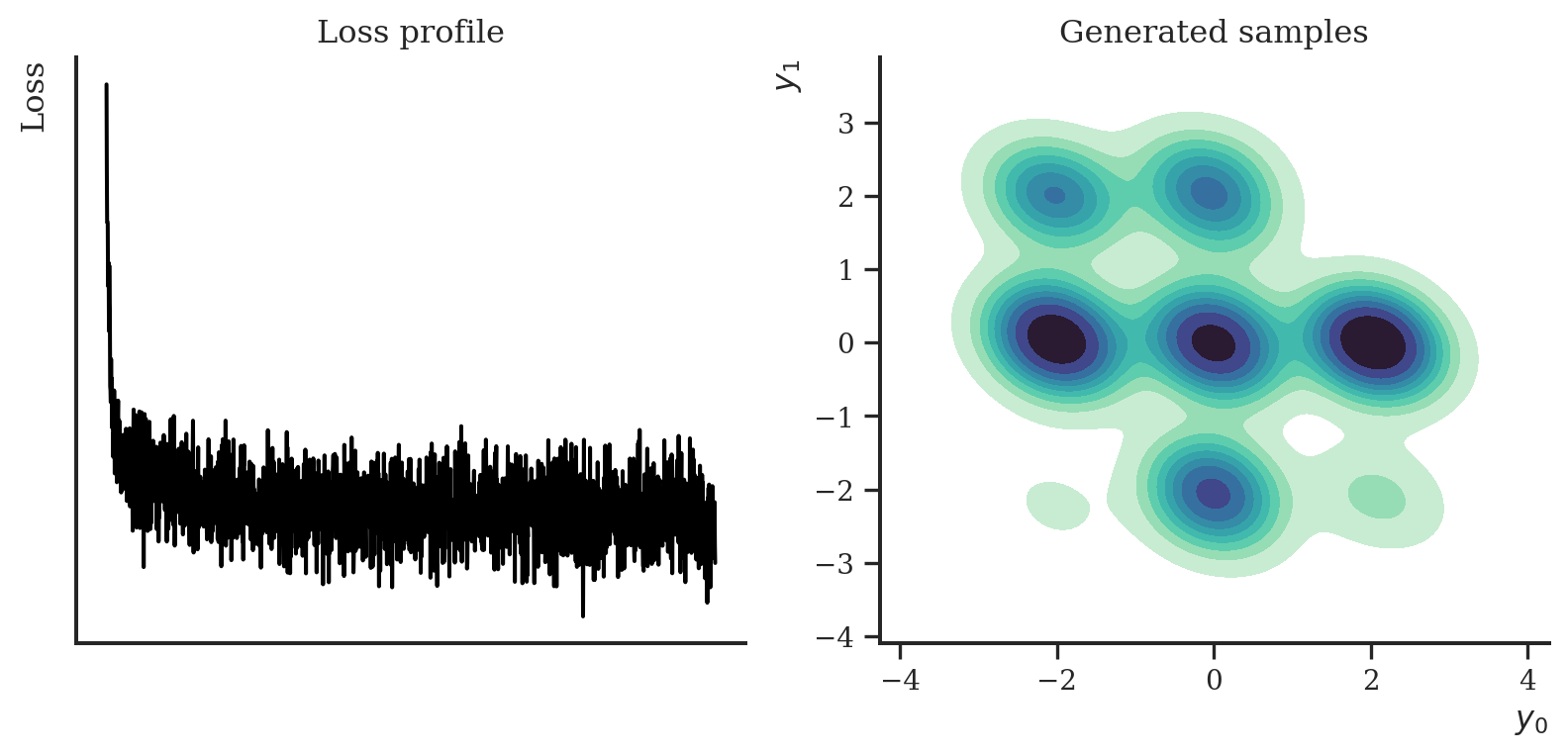
Having trained the model, let’s visualize the trace of the loss and draw some samples. The samples should look similarly to the original data set, the 9 Gaussians.

Code

samples = model.apply(
    params, random.PRNGKey(0), method="sample", sample_shape=(1000,), n=100, eps=2e-5
)

def plot(losses, samples):
    fig, (ax1, ax2) = plt.subplots(1, 2, figsize=(10, 4))
    sns.lineplot(
        data=pd.DataFrame({"y": np.asarray(losses), "x": range(len(losses))}),
        y="y",
        x="x",
        color="black",
        ax=ax1
    )
    sns.kdeplot(
        data=pd.DataFrame(np.asarray(samples), columns=["x", "y"]),
        x="x",
        y="y",
        fill=True,
        cmap="mako_r",
        ax=ax2
    )
    ax1.set(title="Loss profile", xlabel="", ylabel="Loss", xticks=[], xticklabels=[], yticks=[], yticklabels=[])
    ax2.set(title="Generated samples", xlabel="$y_0$", ylabel="$y_1$")
    plt.show()

plot(losses, samples)

DDPM

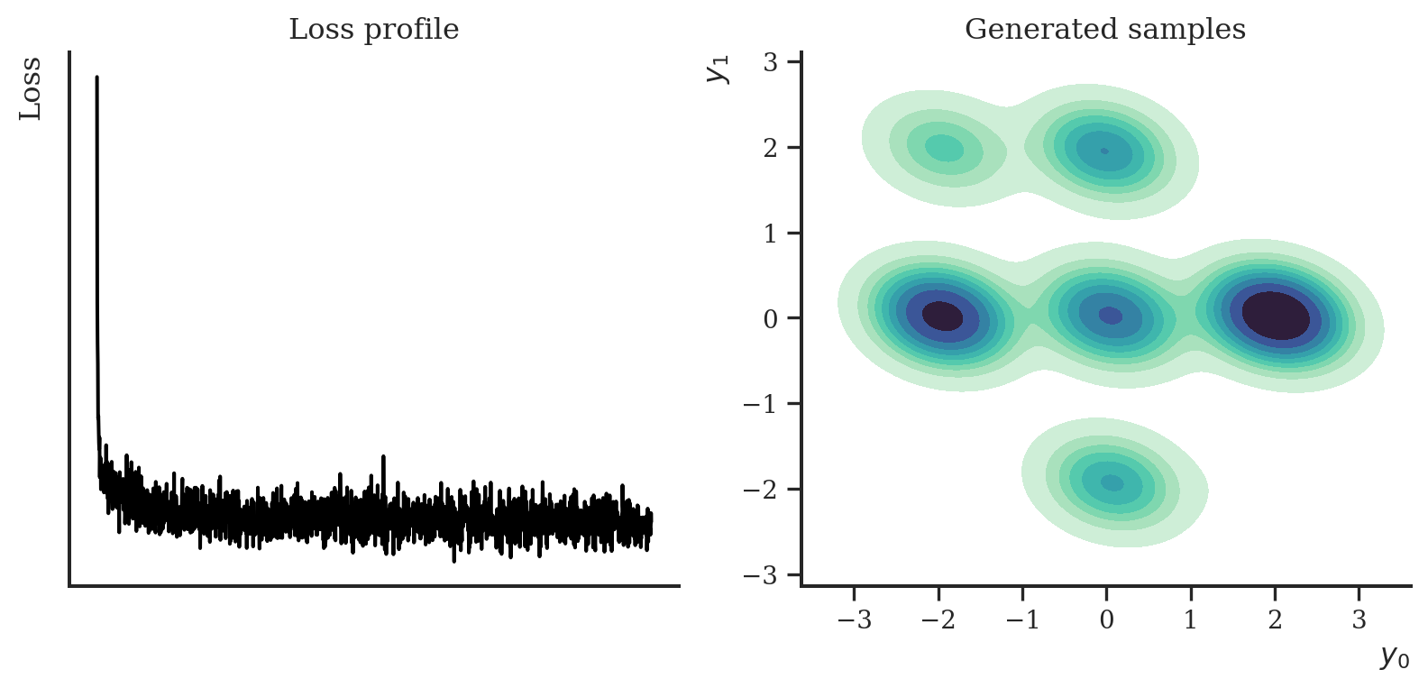
The DDPM implementation looks almost identical. Instead of a noise schedule, we supply a vector of \(\beta\)s. In comparison to the NCSN, we don’t need to use Langevin dynamics to sample new data, but can run the Markov chain in reverse. Here, we choose to use the parameterization from the paper which predicts the noise \(\boldsymbol \epsilon\) that is used to generate a latent variable \(\mathbf{y}_t\), but it is equivalent to predicing the mean of the forward process posterior.

class DDPM(hk.Module):
    def __init__(self, score_model, betas):
        super().__init__()
        self.score_model = score_model
        self.n_diffusions = len(betas)
        self.betas = betas
        self.alphas = 1.0 - self.betas
        self.alphas_bar = jnp.cumprod(self.alphas)
        self.sqrt_alphas_bar = jnp.sqrt(self.alphas_bar)
        self.sqrt_1m_alphas_bar =jnp.sqrt(1.0 - self.alphas_bar)

    def __call__(self, method="loss", **kwargs):
        return getattr(self, method)(**kwargs)

    def loss(self, y, is_training=True):
        t = random.choice(
            key=hk.next_rng_key(),
            a=jnp.arange(0, self.n_diffusions),
            shape=(y.shape[0],),
        ).reshape(-1, 1)
        noise = random.normal(hk.next_rng_key(), y.shape)
        perturbed_y = (
            self.sqrt_alphas_bar[t] * y +
            self.sqrt_1m_alphas_bar[t] * noise
        )
        eps = self.score_model(
            perturbed_y,
            t.reshape(-1),
            is_training,
        )
        loss = jnp.sum(jnp.square(noise - eps), axis=-1)
        return loss

    def sample(self, sample_shape=(1,)):
        def _fn(i, x):
            t = self.n_diffusions - i
            z = random.normal(hk.next_rng_key(), x.shape)
            sc = self.score_model(
                x,
                jnp.full(x.shape[0], t),
                False,
            )
            xn = (1 - self.alphas[t]) / self.sqrt_1m_alphas_bar[t] * sc
            xn = x - xn
            xn = xn / jnp.sqrt(self.alphas[t])
            x = xn + self.betas[t] * z
            return x
        
        z_T = random.normal(hk.next_rng_key(), sample_shape + (2,))
        z0 = hk.fori_loop(0, self.n_diffusions, _fn, z_T)
        return z0

Just as in the original publication, we define a \(\beta\)-schedule a linear sequence.

def _ddpm(**kwargs):
    score_model = ScoreModel()
    model = DDPM(score_model, jnp.linspace(10e-4, 0.02, 100))
    return model(**kwargs)


model = hk.transform(_ddpm)
params = model.init(random.PRNGKey(0), y=y)

Let’s again optimize this and generate some new data.

optimizer = optax.adamw(0.001)
opt_state = optimizer.init(params)

params, losses = optim(params, opt_state)
losses = jnp.asarray(losses)

Code

samples = model.apply(params, random.PRNGKey(0), method="sample", sample_shape=(1000,))
plot(losses, samples)

Score-based SDE

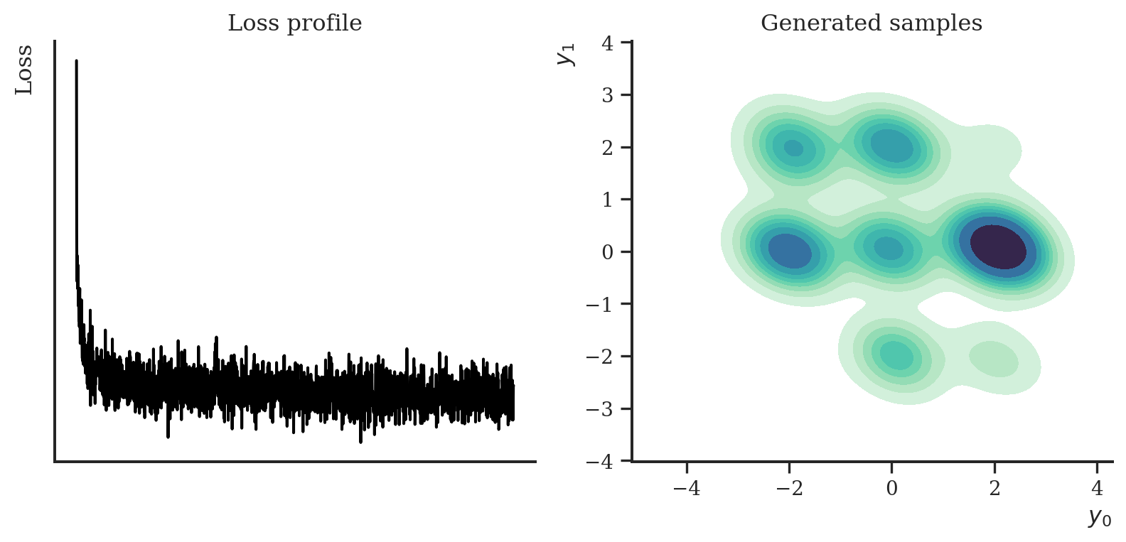
Finally, we implement a continuous-time diffusion model using stochastic differential equations. Again, the base implementation is fairly similar to the models before. The only thing we have to adapt in comparison to the NCSN is that we now provide a function that computes the mean and standard deviation for the transition kernel \(p_{st}(\mathbf{y}(t) \mid \mathbf{y}(s))\) and one function that computes the drift and diffusion coefficients of the forward and reverse SDEs (which are identical in both directions).

Here, for some variate we will choose the sub variance-preserving SDE from the original publication:

\[\begin{align*} \mathrm{d} \mathbf{y} & = \mathbf{f}(\mathbf{y}, t) \mathrm{d}t + g(t)\mathrm{d}\mathbf{w} \\ & = - \frac{1}{2} \beta(t)\mathbf{y}\mathrm{d}t + \sqrt{\beta{t}(1-\exp(-2 \smallint_0^t \beta(s) \mathrm{d}s))} \mathrm{d}\mathbf{w} \end{align*}\]

The respective transition kernel is given by

\[\begin{align*} p_{0t}(\mathbf{y}(t) \mid \mathbf{y}(0)) = \mathcal{N}\left( \mathbf{y}_0 \exp \left( -\tfrac{1}{2}\smallint_0^t\beta(s) \mathrm{d}s \right), \left[1 - \exp \left( -\tfrac{1}{2}\smallint_0^t \beta(s) \right) \mathrm{d}s \right]^2\mathbf{I} \right) \end{align*}\]

The implementations of the SDE and a function that computes the mean and standard deviation of the transition kernel are shown below:

from functools import partial

def beta_fn(t, beta_max, beta_min):
    return beta_min + t * (beta_max - beta_min)

def integral(t, beta_max, beta_min):
    return beta_min*t + 0.5 * (beta_max - beta_min) * t**2

def sde(x, t, beta_max, beta_min):
    beta_t = beta_fn(t, beta_max, beta_min)
    intr = integral(t, beta_max, beta_min)
    drift = -0.5 * x * beta_t
    diffusion = 1.0 - jnp.exp(-2.0 * intr)
    diffusion = jnp.sqrt(beta_t * diffusion)
    return drift, diffusion

def p_mean_scale(x, t, beta_max, beta_min):
    intr = integral(t, beta_max, beta_min)
    mean = x * jnp.exp(-0.5 * intr)[:, None]
    std = 1.0 - jnp.exp(-intr)
    return mean, std

p_mean_scale_fn = partial(p_mean_scale, beta_min=0.1, beta_max=10.0)
sde_fn = partial(sde, beta_min=0.1, beta_max=10.0)

The constructor of the score-based SDE takes the score model, the function that computes the parameters of the transition kernel and the SDE itself.

class ScoreSDE(hk.Module):
    def __init__(self, score_model, p_mean_scale, sde):
        super().__init__()
        self.score_model = score_model
        self.T = 1.0
        self.p_mean_scale = p_mean_scale
        self.sde = sde

    def __call__(self, method="loss", **kwargs):
        return getattr(self, method)(**kwargs)

    def loss(self, y, is_training=True, eps=1e-8):
        def _log_pdf(y, mu, scale):
            scale = jnp.full(mu.shape, scale)
            return distrax.MultivariateNormalDiag(mu, scale).log_prob(y)
        
        t = jax.random.uniform(
            hk.next_rng_key(), (y.shape[0],), minval=eps, maxval=self.T
        ).reshape(-1)
        z = jax.random.normal(hk.next_rng_key(), y.shape)
        mean, scale = self.p_mean_scale(y, t)
        perturbed_y = mean + z * scale[:, None]
        score = self.score_model(perturbed_y, t, is_training)
        loss = jnp.sum((score * scale[:, None] + z) ** 2, axis=-1)
        return loss

    def sample(self, sample_shape=(1,), is_training=False, eps=1e-8):
        z = jax.random.normal(hk.next_rng_key(), sample_shape + (2,))
        _, scale = self.p_mean_scale(y, jnp.atleast_1d(self.T))
        x_init = z * scale

        def ode_func(t, x):
            x = x.reshape(-1, 2)
            drift, diffusion = self.sde(x, jnp.atleast_1d(t))
            t = np.full((x.shape[0],), t)
            score = self.score_model(x, t, is_training)
            ret = drift - 0.5 * (diffusion**2) * score
            return ret.reshape(-1)

        res = integrate.solve_ivp(
            ode_func,
            (self.T, eps),
            np.asarray(x_init).reshape(-1),
            rtol=1e-5,
            atol=1e-5,
            method="RK45",
        )

        return res.y[:, -1].reshape(x_init.shape)

Let’s test the score-based SDE. We use the same procedure as above and again train with AdamW.

def _score_sde(**kwargs):
    score_model = ScoreModel()
    model = ScoreSDE(score_model, p_mean_scale_fn, sde_fn)
    return model(**kwargs)

model = hk.transform(_score_sde)
params = model.init(random.PRNGKey(0), y=y)

optimizer = optax.adamw(0.001)
opt_state = optimizer.init(params)

params, losses = optim(params, opt_state)
losses = jnp.asarray(losses)

Let’s again draw some samples and look at the loss profile.

Code

samples = model.apply(params, random.PRNGKey(0), method="sample", sample_shape=(1000,))
plot(losses, samples)

Conclusion

This case study implemented three recent developments in generative diffusions. We first implemented the NCSN and DDPM objectives, and then the framework by Song et al. (2021) which turned out to be a continuous time generalisation of both models. In terms of sample quality, for the nine Gaussians data set the results are somewhat similar.

Session info

import session_info
session_info.show(html=False)

-----
arviz               0.12.0
distrax             0.1.2
haiku               0.0.9
jax                 0.4.5
jaxlib              0.4.4
matplotlib          3.6.2
numpy               1.24.2
optax               0.1.3
palettes            NA
pandas              1.5.1
scipy               1.10.1
seaborn             0.11.2
session_info        1.0.0
-----
IPython             8.4.0
jupyter_client      7.3.4
jupyter_core        4.10.0
jupyterlab          3.3.4
notebook            6.4.12
-----
Python 3.9.10 | packaged by conda-forge | (main, Feb  1 2022, 21:27:43) [Clang 11.1.0 ]
macOS-13.0.1-arm64-i386-64bit
-----
Session information updated at 2023-03-04 13:09

License

The case study is licensed under a Creative Commons Attribution-NonCommercial 4.0 International License.

References

Anderson, Brian DO. 1982. “Reverse-Time Diffusion Equation Models.” Stochastic Processes and Their Applications 12 (3): 313–26.

Ho, Jonathan, Ajay Jain, and Pieter Abbeel. 2020. “Denoising Diffusion Probabilistic Models.” Advances in Neural Information Processing Systems 33: 6840–51.

Hyvärinen, Aapo, and Peter Dayan. 2005. “Estimation of Non-Normalized Statistical Models by Score Matching.” Journal of Machine Learning Research 6 (4).

Sohl-Dickstein, Jascha, Eric Weiss, Niru Maheswaranathan, and Surya Ganguli. 2015. “Deep Unsupervised Learning Using Nonequilibrium Thermodynamics.” In International Conference on Machine Learning, 2256–65. PMLR.

Song, Yang, and Stefano Ermon. 2019. “Generative Modeling by Estimating Gradients of the Data Distribution.” Advances in Neural Information Processing Systems 32.

Song, Yang, Jascha Sohl-Dickstein, Diederik P Kingma, Abhishek Kumar, Stefano Ermon, and Ben Poole. 2021. “Score-Based Generative Modeling Through Stochastic Differential Equations.” In International Conference on Learning Representations.

Vincent, Pascal. 2011. “A Connection Between Score Matching and Denoising Autoencoders.” Neural Computation 23 (7): 1661–74.